Scheduled Statistics
Hopsworks scheduled statistics allows you to monitor your feature data once they have been ingested into the Feature Store. You can define a detection window over your data for which Hopsworks will compute the statistics on a regular basis. Statistics can be computed on all or a subset of feature values, and on one or more features simultaneously.
Hopsworks stores the computed statistics and enable you to visualise the temporal evolution of statistical metrics on your data.
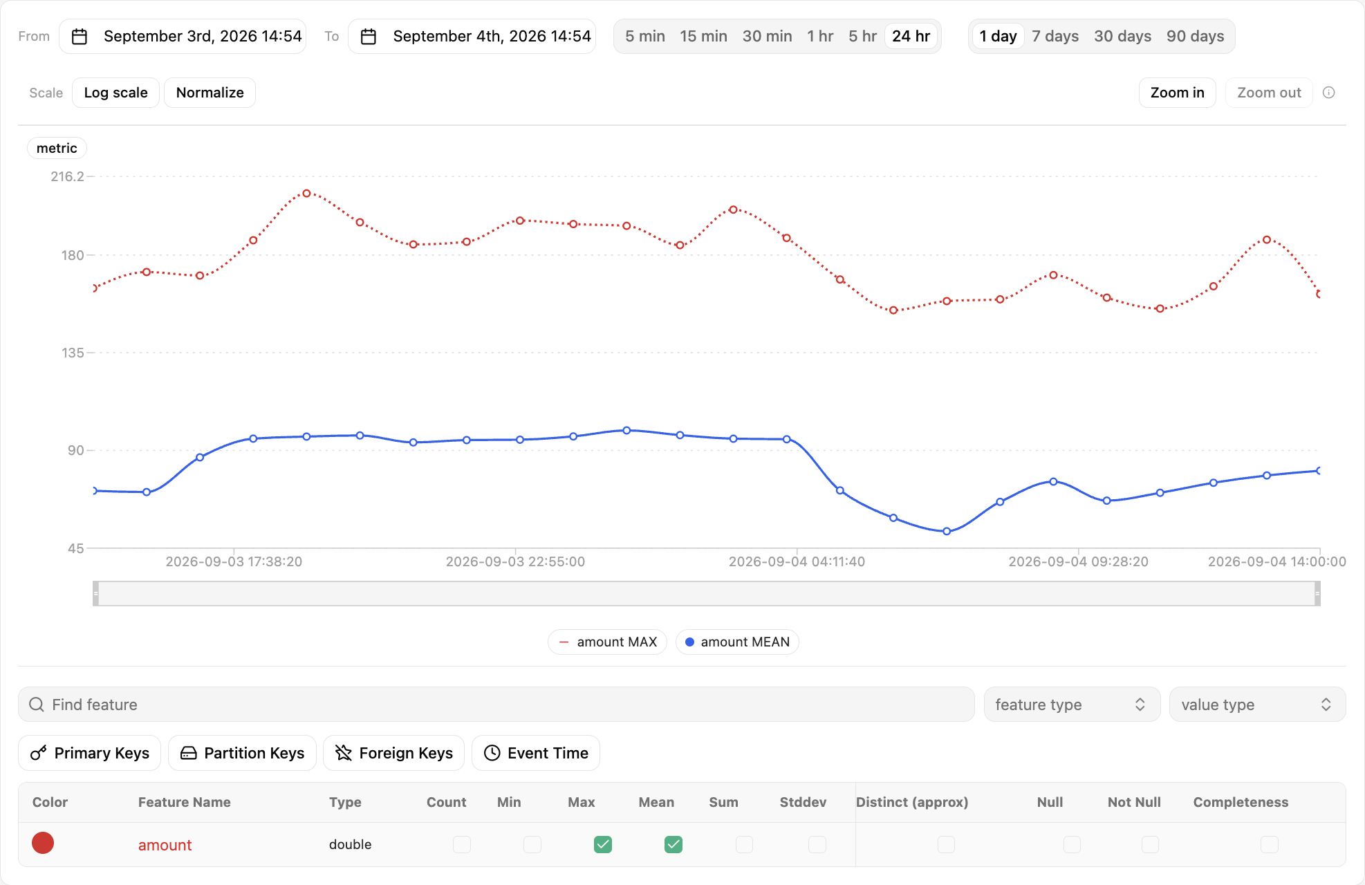
Interactive graph
See the Interactive graph guide to learn how to explore statistics more efficiently.
Use cases#
Scheduled statistics monitoring is a powerful tool that allows you to monitor your data over time and detect anomalies in your feature data at a glance by visualizing the evolution of the statistics properties of your data in a time series. It can be enabled in both Feature Groups and Feature Views, but for different purposes.
For Feature Groups, scheduled statistics enables you to analyze how your Feature Group data evolve over time, and leverage your intuition to identify trends or detect noisy values in the inserted feature data. See the Feature Monitoring for Feature Groups guide to configure it.
For Feature Views, scheduled statistics enables you to analyze the statistical properties of potentially new training dataset versions without having to actually create new training datasets and, thus, helping you decide when your training data show sufficient significant changes to create a new version. See the Feature Monitoring for Feature Views guide to configure it.
Detection windows#
Statistics are computed in a scheduled basis on a pre-defined detection window of feature data. Detection windows can be defined on the whole feature data or a subset of feature data depending on the time_offset and window_length parameters of the with_detection_window method.
In a previous section we described different types of windows available. Taking a Feature Group as an example, the figure above describes how these windows are applied to Feature Group data, resulting in three different applications:
- A expanding window covering the whole Feature Group data from its creation until the time when statistics are computing. It can be seen as an snapshot of the latest version of your feature data.
- A rolling window covering a variable subset of feature data (e.g., feature data written last week). It helps you analyze the properties of newly inserted feature data.
Time basis#
A rolling window needs a notion of time to decide which rows fall inside it. Hopsworks supports two bases, chosen once per configuration and shared by the detection and reference windows:
- Event time: rows are selected by the value of an event-time feature, so a window such as "last week" contains the rows whose event time falls in that week regardless of when they were written. This is the default for Feature Groups and Feature Views that declare an
event_time. - Commit time: rows are selected by the time they were written to the Feature Group, using time travel. A window such as "last week" contains the rows committed during that week. This is the default when no event-time feature is declared, and it requires a time-travel enabled Feature Group.
A rolling event-time window is anchored on the time the schedule fires. Each run selects the rows whose event time is inside the window at that moment and stores their statistics.
A row that lands after the run covering its event time is not added to that run's statistics, and every later window starts after its event time, so no window counts it. This happens with backfills and with the materialization lag of streaming pipelines. For backfill-heavy pipelines, use an expanding window, which has no lower bound, or the commit-time basis, which selects rows by when they were written.
Leave room for late rows
time_offset sets where the window starts, counted back from the run, and window_length sets how long it lasts, so a time_offset longer than the window_length ends the window before the run. For example, a daily schedule with time_offset="25h" and window_length="24h" that runs at 12:00 on Tuesday covers event times from 11:00 on Monday to 11:00 on Tuesday, and the next run covers 11:00 on Tuesday to 11:00 on Wednesday. Consecutive windows meet, and each row has one hour to land before the window that covers it runs. Size the gap to the longest delay with which rows land, such as the materialization interval of the pipeline.
Updated rows
An event-time window reads the current snapshot of the data and filters it on the event-time feature, so it sees only the latest version of each row. A commit-time window reads the commits in its range, so each version of an updated row is counted in the window of the commit that wrote it.
See more details on how to define a detection window for your Feature Groups and Feature Views in the Feature Monitoring Guides for Feature Groups and Feature Views.
Next steps
You can also define a reference window to be used as a baseline to compare against the detection window. See more details in the Statistics comparison guide.